National 5 Physics

Acceleration

Acceleration is the change in velocity divided by the time it took to make that change. Another way of stating this is to say that acceleration is the rate of change of velocity. To measure acceleration we need to know the starting velocity, u, the final velocity, v, and the time between these two measurements. The equation relating these quantities together is:

$$a=\frac{\mathrm{(v\; -\; u)}}{t}$$

Example

A cart is moving down a ramp and the initial speed is measured as 1.0 m s^-1. At the bottom of the ramp the speed is 4.0 m s^-1. The time between the two measurements was 1.5 seconds. What was the acceleration of the cart?
u = 1.0 m s^-1
v = 4.0 m s^-1
t = 1.5 s
a = ?

$$a=\frac{\mathrm{(v\; -\; u)}}{t}$$ $$a=\frac{\mathrm{(4.0\; -\; 1.0)}}{\mathrm{1.5}}$$ $$a={\mathrm{2.0\; m\; s}}^{\mathrm{-2}}$$

Example

A car accelerates at 3.0 m s^-2 for 5.0 seconds. The final velocity is 17 m s^-1. What was the initial velocity of the car?
u = ?
v = 17 m s^-1
t = 5.0 s
a = 3.0 m s^-2

$$a=\frac{\mathrm{(v\; -\; u)}}{t}$$ $$\mathrm{3.0}=\frac{\mathrm{(17\; -\; u)}}{\mathrm{5.0}}$$ $$u={\mathrm{2.0\; m\; s}}^{\mathrm{-1}}$$

Example

How long would it take a car to slow from 15 m s^-1 to rest if the acceleration has a magnitude of 3.75 m s^-2?
u = 15 m s^-1
v = 0.0 m s^-1
t = ? s
a = -3.75 m s^-2
NOTE: The sign in front of the acceleration is negative because it is acting in the opposite direction to the motion of the car.

$$a=\frac{\mathrm{(v\; -\; u)}}{t}$$ $$\mathrm{-3.75}=\frac{\mathrm{(0\; -\; 15)}}{t}$$ $$t=\mathrm{4.0\; s}$$

---

Interactive example 1 and solution

Try and solve the question before clicking the solve button to check your answer

A car is travelling at m s^-1. Ater accelerating at a constant rate for seconds it has a velocity of m s^-1. What is the acceleration experienced by the car?

---

Interactive example 2 and solution

Attempt to solve the question yourself before clicking the solve button!

A skier is coming to the end of their run. They are travelling at m s^-1 when they begin to slow down. How long will it take them to stop if they are accelerating at m s^-2 ? (Hint:remember that this value must be negative)

---

Interactive example 3 and solution

Try and solve the question before clicking the solve button to check your answer

A lorry is travelling at m s^-1 when it accelerates at a constant value of m s^-2. How fast will the lorry be travelling if the acceleration lasts for s?

---

Acceleration from velocity-time graph

In this section we will use the following graph, with its numbered regions to determine the acceleration of the object.

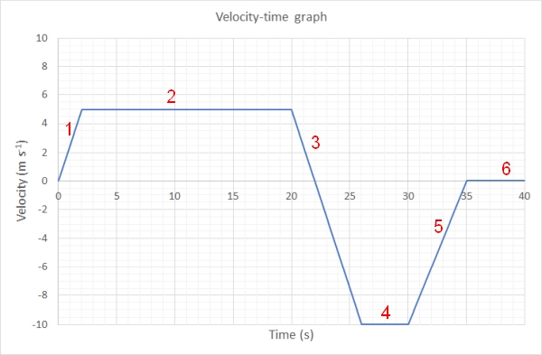
The first part of the v-t graph shows an acceleration because the line on the graph is a diagonal. To calculate the acceleration at this point we need to work out the gradient of this line.
The gradient of a line requires two points on the line and the following equation:

$$m=\frac{y_2-y_1}{x_2-x_1}$$

From the graph we have the following two points (0,0) and (2,5)

$$m=\frac{y_2-y_1}{x_2-x_1}$$ $$m=\frac{5-0}{2-0}$$ $$m={\mathrm{2.5\; m\; s}}^{\mathrm{-2}}$$

Therefore the acceleration of the object at the start of the graph is 2.5 m s^-2.

In the third section of the graph there is also an acceleration. The two points for this line are (20,5) and (25, -10).

$$m=\frac{y_2-y_1}{x_2-x_1}$$

From the graph we have the following two points (0,0) and (2,5)

$$m=\frac{y_2-y_1}{x_2-x_1}$$ $$m=\frac{\mathrm{-10}-5}{\mathrm{25}-\mathrm{20}}$$ $$m={\mathrm{-3.0\; m\; s}}^{\mathrm{-2}}$$

Notice that the value of the acceleration is negative, indicating it is in the opposite direction to the movement of the object. That is until the velocity becomes negative, and then it continues to speed up in the opposite direction reaching a backwards velocity with a magnitude of 10 m s^-1.

The 5th section of the graph is also an acceleration. The value of the acceleration is 2.0 m s^-2. You should attempt to solve this and see if you get this answer.

Experimental determination of acceleration

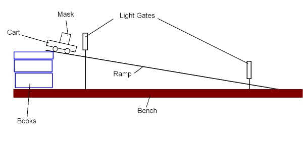
The determination of acceleration is commonly found using light gates and a datalogger. There are two possible setups depending on the type of information required.

Where two light gates are used with a separation of 1.0 metre the average acceleration is determined.
Where a single light gate with a double mask is used the value of acceleration is accepted as the instantaneous acceleration.

Average Acceleration

In the animation below if the cart is at the bottom of the ramp just move the mouse over the title of the experiment to reset the animation

From the above diagram and animation we can see that the mask will cut the beam for the light gate. If we input the width of the mask into the datalogger it will calculate the velocity of the cart at each light gate. The student needs to measure the time the cart takes to travel between the two light gates. The result table for an experiment carried out by this technique is given below.

Run number	Initial velocity (m s-1)	Final velocity (m s-1)	Time between light gates (s)
1	0.25	1.13	1.25
2	0.27	1.08	1.26
3	0.24	1.10	1.24
Average	0.25	1.10	1.25

The acceleration can be clalculated from the average values:

$$a=\frac{\mathrm{(v\; -\; u)}}{t}$$ $$a=\frac{\mathrm{(1.10\; -\; 0.25)}}{\mathrm{1.25}}$$ $$a={\mathrm{0.68\; m\; s}}^{\mathrm{-2}}$$

So this gives the average acceleration of the cart down the ramp as 0.68 m s^-2.

Average Acceleration Experiment

Now it is your turn to carry out a virtual experiment. This requires flash which is installed on the server and should run in any modern browser

 

Average Acceleration Experiment

Instantaneous Acceleration

In order to find the instantaneous acceleration we only need to use one light gate and a double mask. With the length of each part of the double mask the datalogger will caclulate and display directly the acceleration of the cart.

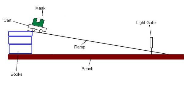
The U shaped mask provides the datalogger with the three pieces of information that it needs to work out the acceleration.
1) The first time the light gate is blocked the datalogger can calculate a value for the initial speed (u)
2) The next piece of information is the time gap between the first blocking of the light gate and the second blocking by the back part of the mask (t)
3) The third piece of information is the final velocity from the blocking of the light gate by the back part of the mask (v)
Software in the datalogger carries out the calculation

It then displays the value for acceleration (a) on the display.

Clearly this requires a machine to make the measurements because human reaction times are too large for such small measurements of time.

 

$$a=\frac{\mathrm{(v\; -\; u)}}{t}$$

 

In the animation below if the cart is at the bottom of the ramp just move the mouse over the title of the experiment to reset the animation