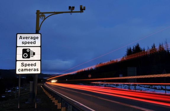
Average Speed
In the recent past averge speed cameras have been installed on the main road between Aberdeen and Dundee. They are there to make sure that drivers stay below the speed limit for a long part of this road. How do we calculate average speed?
This comes from knowing the distance travelled and the time taken to go that distance. The equation that we use is:
Where
d = distance travelled
v = speed
t = time taken to go the distance
Example:
A car travels 150 km in a time of 2 hours. What is its average speed?
d = 150 km
v = ?
t = 2 hours
Notice that when dealing with speeds like this we do not have to convert to metres per second, as kilometres per hour is widely used. In the laboratory when we do experiments the speed will be calculated in metres per second because these will be the units we are measuring in.
How long did it take to travel that far?
Attempt to solve the question yourself before clicking the solve button!
Average Velocity Experiment
Below is a short animation of a key experiment. The details of the experiment are given below. The velocity is determined over a relatively long distance (1.00 m) and so we refer to it as an average velocity.
If the cart is at the bottom of the ramp move the cursor over the title of the experiment to reset it.
- Measure accurately the distance between the two light gate sensors
- Set the data logger to measure the time gap between the two light gates being interrupted.
- Use the manufacturer's instructions to set the details on the datalogger
- Release the cart from a specified point on the ramp
- Repeat the experiment and determine the average time it takes for the card to pass between the gates
- Using the data for distance and time determine the average velocity of the cart
- When the card blocks the first light gate the timer switches on
- When the card blocks the second light gate the timer switches off, which gives the values in the table below.
The times recorded by the datalogger were:
| Trial | 1 | 2 | 3 | 4 | 5 |
|---|---|---|---|---|---|
| Time (s) | 1.25 | 1.28 | 1.27 | 1.22 | 1.23 |
Instantaneous Velocity
In the experiment above the velocity at the top of the ramp and the bottom of the ramp may have been different, but that experiment could only determine the average velocity across the 1.00 m distance.
How can we determine the velocity in an instant? We need to have a much shorter time interval to measure the distance travelled. Our manual timing skills are to slow for this short time interval. Therefore, in this experiment there is one light gate. It will measure the time it takes for the 5.0 cm to cut the beam. This extremely short time is only measurable by a machine.
In the animation below you can see the setup for an instantaneous velocity experiment.
- Carefully measure the width of a card that you attatch to the cart.
- In this experiment it is 5.0 cm
- Setup a light gate at the bottom of the ramp
- Set the data logger to time how long the light gate is blocked or to the speed setting
- Use the manufacturer's instructions to set the details on the datalogger
- Release the cart from a specified point on the ramp
- Repeat the experiment and determine the average time it takes for the card to pass through the gate
If the cart is at the bottom of the ramp move the mouse over the title to reset the animation.
In the instantaneous velocity experiment the following times were recorded
| Trial | 1 | 2 | 3 | 4 | 5 |
|---|---|---|---|---|---|
| Time (s) | 0.043 | 0.047 | 0.046 | 0.044 | 0.045 |
This gives an average time of 0.045 s for the 5.0 cm card to pass through the light gate.
So we can see that the instantaneous velocity of the cart at the bottom of the ramp was 1.1 m s-1.
Average Velocity Experiment
Gap-fill exercise
Velocity-time graphs
In the table below are the three possible motions of an object.
- The first graph shows the object at rest.
- The second graph shows the object moving at a constant velocity in the positive direction. This is often a problem when dealing with these graphs. Velocity is a vector quantity and therefore must include direction. Quite often the default is the object moving to the right is moving in a positive direction. In this case if the object moves to the left at a constant velocity the horizontal line on the graph would be below the x-axis.
- The third graph shows a constant acceleration. Acceleration is also a vector quantity and so using the default of motion to the right being positive, this means that the object is accelerating to the right. A deceleration, or an acceleration to the left would be a diagonal line sloping in the opposite direction.
| Stationary | Constant velocity | Constant acceleration | |
|---|---|---|---|
| velocity-time | 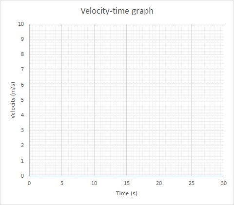 |
 |
 |
Hovering over a graph in the table will enlarge it
Example
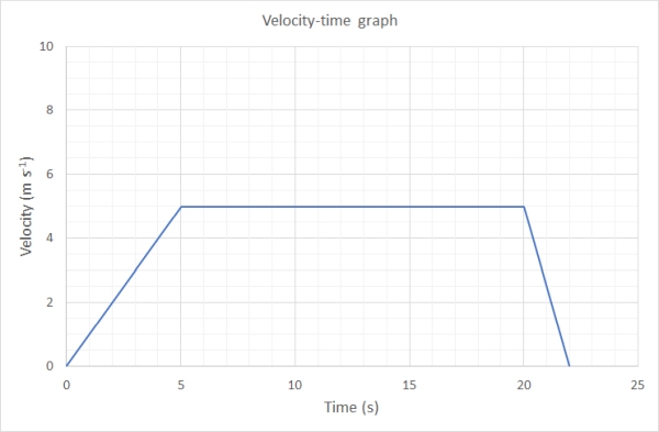
A cyclist is at rest at some traffic lights. She then acelerates uniformly at 1 m s-1 for 5 seconds. The cyclist then travels at a constant velocity of 5 m s-1 for 15 seconds. They then brake and comes to a rest in 2 seconds. Draw a graph of this journey.
The distance the bike travelled in this time can be determined by working out the area under the graph. This is given by calcuating the area of the two triangles (A & C) and the rectangle (B) between them and adding these all together.
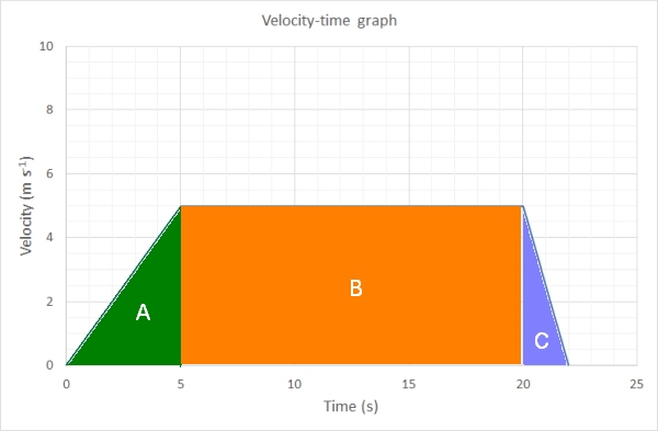
The area of a triangle is 1/2 base × height
Triangle A area = 1/2 × 5 × 5 = 12.5 m
Triangle C area = 1/2 × 5 × 2 = 5 m
Rectangle B area = 5 × 15 = 75 m
Total area = 12.5 + 5 + 75 = 92.5 m
Therefore the distance travelled by the bike is 92.5 m
Example
Describe the motion of the object in the folowing graph
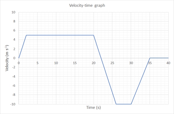
First let us break the graph into the six different sections as can be seen on the graph below:
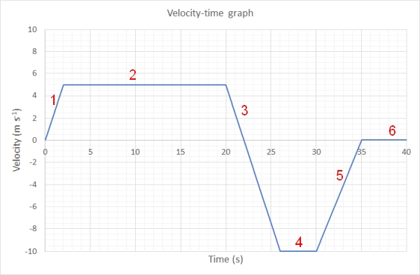
- The object starts at rest and accelerates uniformly at 2.5 m s-2 for 2 seconds (between 0 and 2 seconds)
- The object then travels at a constant velocity of 5 m s-1 (between 2 and 20 seconds)
- The object then uniformly accelerates in the opposite direction at -3.0 m s-2 (between 20 and 25 seconds)
- The object then moves backwards at -10 m s-1 for 5 seconds (between 25 and 30 seconds)
- The object then uniformly accelerates in the forward direction at + 2 m s-2 (which actaully means it is slowing down in its backwards velocity) until it comes to rest (between 30 and 35 seconds)
- The object remains at rest for 5 seconds (between 35 and 40 seconds)